Reditus ad propositum

The diggresio is an aversio ad rem. The return to main topic after a digressio. Involves a 'continual ongoing consciousness and articulation of structure'.

From Sonnino, 156:

Cicero: a neat and elegant return to the main theme after a digression
Wilson: When we have made a digression, we may declare our return... we will now keep us within our bounds.

In Chaucer:

"There as I left I will again begin" in line 35 of Knight's Tale

Another example in John Knox:

"Now to your argument...." and "but omitting..."

The antecedent to the digression would be, according to Quintilian (9.2.55-57), the aposiopesis which in some instances could be used as a transitional device to introduce a digressio or announce an impromptu change in the line of argument. (See The Princeton Encyclopedia of Poetry and Poetics: 4th Ed., p. 61).

Other candidates to announce a digressio are (from Sonnino, 247-248):

• Metabasis (Transitio): See the nice entry with examples from Peacham's The Garden of Eloquence here.
• Apostrophe
• Prosodiasaphesis
• Interjectio
• Improvisum

References:

Sonnino, L. (1968) A Handbook of Sixteenth Centrury Rhetoric. Barnes & Noble,
Holton, A. (2008) The Sources of Chaucer's Poetics. Ashgate. 74ff
Farrow, K. (1990) Humor, Logic, Imagery and Sources in the Prose Writings of John Knox. Studies in Scottish Literature. 25, 1, 154-175. here
Elliot, R. (1919) Transition in the Attic Orators. The Collegiate Press. here

Python in ArcGis / IF - ELSE statements

1) Write the function in the "Show Codeblock" area
2) Invoke it in the definition area
Remember: 2 and 4 spaces indentation for Python...

Autocorrect file in MS Word 2003

My Autocorrect File in MS Word, wasn't updating automatically as I added new entries (Alt-T, A). Each time I entered a term, a Message with Chinese characters appeared. So, I searched the MSO1033.acl file which has the English US autocorrect file, opened it in WordPad and saved it. After that, MS Word has updated each time I add a new entry. Here's a list of the most used .acl files:

English U.S. 1033 (&H409) (e.g. MSO1033.acl)

English U.K. 2057 (&H809)

And the most popular Spanish:

Spanish (Traditional) 1034 (&H40A)
Spanish Argentina 11274 (&H2C0A)
Spanish Spain (Modern Sort) 3082 (&HC0A)

Check the other files here:
http://support.microsoft.com/?kbid=221435

Disclaimer: I know, I prefer Latex too :-)

General Helps

1) If you forget the password of a MS Word file, here's what you can do:
a) Save your file as .rtf
b) open the .rtf file and go to Tools>Options>Security and press Unprotect Document.
c) Do your changes
d) Save file as .doc again


2) How to change font size in MS Word "Document map"?
a) Open Format/Styles and Formatting
b) Select the dropdown menu "Show" and choose "Custom..."
c) In "Styles to be visible", check "Document Map". OK
d) Go to Styles and Formatting again and select Document Map and change the font.

Handout of Adobe Illustrator

Here's a couple of frequently-needed hints to work in Illustrator:

1) Faded edges on a picture: Select image, Effect>Stylize>Feather then choose radius
2) 3D effect on text: Select text, Effect>3D>Extrude and Bevel> Set options as desired
3) Group: Select and Ctrl+G or Select, Object>Group
4) Trim a picture: draw rectangle upon figure, Select both rectangle and figure (Shift+click), go to Object>Clipping Mask>Make. More here

Good source of general info:

http://help.adobe.com/en_US/illustrator/cs/using/WS714a382cdf7d304e7e07d0100196cbc5f-62f2a.html

Solving Linear Programming problems with several constraint types in Matlab

The most difficult part of linear programming is the model building. However, once the model is clearly stated, the constraints may be a challenge. It might be the case that some constraints are less than some constant while others are larger than some constant, and even other are equal to a coefficient. In addition, it is important to keep in mind that the Matlab routine linprog is devised to solve minimization problems, not maximization. So before solving the problem, we have to make sure that all the constraints and equalities, etc. are consistent with the input structure of linprog in Matlab. In order to show this I prepared a short handout and I also work a textbook example for illustration purposes.
Suppose that we want to minimize an objective function f  subject to the following constraints:

Here we have all the possible constraint cases. Remember that Matlab solves cases in the form:

So we only have to transform the C constraint to , to look like the Matlab formulation. In Matlab code it would look like:

[x,~,~,~,lambda] = linprog(f,[A;-C],[a;c],Beq,beq,lb,ub);

where Beq and beq denote the equality for the B constraint. 
Now let's work a more complicated example from the book Mathematical Models in Agriculture by J.  Thornley and J. France, p. 69-75.
Minimize the following objective function

subject to the following constraints:

A way to solve this in Matlab would be:

f = [6.6 9 36 14.9 65]; f = f(:);
A = [13.7 14.2 11.1 12.3 0;
    108 98 701 503 0;
     .5 .2 79.3 2.3 120;
     3.8 2.7 43.7 10.2 60;
     .2 .1 16.1 5 60;
     1.3 1 2.2 3.1 30];
a = [13 160 7 7 3 2]; b = b(:);
Aeq = [1 1 1 1 1]; % The equality constraint
beq = 1;
lb = [0 .1 0 0 .01]; lb = lb(:); % The lower bounds. Note that  it includes all three at the same time (i.e. x2>.1; x5>.01 and x1,3,4 >= 0) 
[x,~,~,~,lambda] = linprog(f,-A,-a,Aeq,beq,lb);
% Don't forget that to change the sign of Ax>=a both, A and a have to be negative.

Results

x =
      0.74423
          0.1
     0.034488
     0.090751
     0.030536

profit z is:


>> z = f'*x
y_dual = lambda.ineqlin

z =
       10.39
y_dual =
            0
     0.011666
      0.14076
            0
      0.71638
            0

Distance from intersection of two lines to a circle

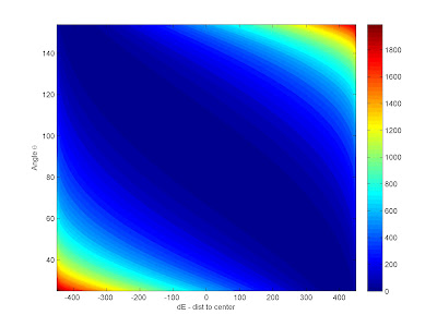
What is the distance from the intersection of two lines to a circle? Here's the graph of the problem with some appropriate notation. So I have to find the distance dW. But to make things more interesting, I want to know dW for several angles of the tangent to the circle (beta) and several positions of the vertical dotted red line (dE). I've tried trigonometry to solve this, but analytic geometry proved much simpler. So, the idea is simply to express the equation of the tangent line as:

 

so using the equation of the line:

The results are displayed in the next graph for all angles and positions of ther vertical line.

Coordinates Transformation

Coordinates transformation simply involves the expression of a coordinate, originally expressed in a coordinate system (2), into a new coordinate system (1). When deriving the coordinates transformation, there is the common way which requires to know a cosine equivalence. As a handout, here's, perhaps, a more intuitive way. 

From the graph

but since: 

we can do:

That can be represented in the usual matrix form:

Create a surface from a 2D function in Matlab

We might be interested in creating a surface from a 2D function. Matlab's command "cylinder", although does something similar, will not be of help for this. Here's how to do it:

"f" function

Suppose we want to revolve a function "f" around the "z" axis. Let's start by defining the range of the "x" axis as:

>> x = 0:10:350;

Next define the range of angles and the number of elements.

>> angs = 0 : 10 : 180;

Now, rotate the axis "x" and "y" by doing:

for i = 1 : length(angs)
    X(:,i) = x * cosd(angs(i));
    Y(:,i) = x * sind(angs(i));
end

We will store the values of "f" in the Z matrix by doing:

>> Z = repmat(f,1,length(angs));

That's it. We now plot the surface with:

surfc(X,Y,Z,'FaceColor','interp',...
    'EdgeColor','none',...
    'FaceLighting','phong')

Here's the result:

Lognormal Parameter Estimation using the mode value and frequency.

If we have to estimate the mean (mu) and standard deviation (sigma) of the lognormal distribution, and we only have the mode available, here's what we can do. I'll show it with an example along with the Matlab code.

Let's say that out mode is occurs at x = 1.5 and its frequency is 10%. Since there's two unkowns, we need two equations. Here's the equation of the lognormal PDF mode:

and here the frequency equation (which happens to be the PDF expression), i.e.:

So, first step is to equal the mode expression to our given value and take logs

Next, substitute in the frequency equation the value of the mode, (i.e. x = 1.5) and the expression of mu as a function of \sigma that we just found in the previous step

Taking logs and simplifying we get:

We can use Matlab to find out the value of \sigma as:

>> solve('-(s^2)^2/(2*s^2)-log(1.5*s*sqrt(2*3.14))=-2.3026')
>> 1.237330637937465265170425634383

We're now good to go with:

All the math is ready now. Let's plot the function with Matlab:

>> x = (.01:20/1000:100)';
>> sig = 1.2373;
>> mu = log(1.5)+sig^2;
>> y = lognpdf(x,mu,sig);
>> semilogx(x,y)

Which is a nice lognormal distribution with mode at x = 1.5 and frequency 10%. 

Finally, we can generalize the above equation as:

where m_l is the mode location and m_f is the mode frequency (from 0 to 1). Once we solve the above equation for sigma, we can find the mean with the following:

Two-Sample t-test (reminder)

The test statistic t0 that we have to calculate from the samples is:

where the y's are sample means, Sp is an estimate of the common variance of both samples

where S1 and S2 are sample variances.

To decide whether to reject H0 or not, we compare the test statistic (the one calculated with the equation above) t0 with another t, from the t-distribution (with n1 + n2 - 2 dof's). If

we have to reject H0 (the second term of the equation is the upper probability alpha/2 of the t-distribution). If this happens, H1 holds.

Reference:

Montgomery, D.G. (2001), Design and Analysis of Experiments. 5th Edition. Wiley.