Review of "An Introduction to Generalized Linear Models, 2nd Edition (Chapman & Hall/CRC Texts in Statistical Science)

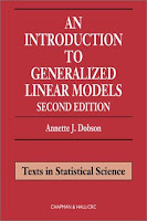
This is a wonderful introductory text to Generalized Linear Models (GLM). The text is crystal clear, concise and practical. There are enough illustrations to explain the concepts. The author does a great job in showing step by step the unity of many statistical techniques that otherwise are often taught unrelated in classrooms. The book helps to visualize the techniques as part of a coherent, interrelated theoretical system. One topic that I didn't find well explained and linked to the whole system is ANOVA in Ch. 6.

Below there are some book exercises solved in Matlab:

Example 4.2: Pressure Vessels. Data is described by a Weibull distribution. Find the parameters of the distribution with the log-likelihood method.

>> data = [1051 1337 1389 1921 1942 2322 3629 4006 4012 4063 4921 5445  5620 5817 5905 5956 6068 6121 6473 7501 7886 8108 8546 8831 9106 9711 9806 10205 10396 10861 11026 11214 11362 11604 11608 11745 11762 11895 12044 13520 13670 14110 14496 15395 16179 17092 17568 17568];
>> [phat,pci] = mle(data,'distribution','wbl','ntrials',4);
>> phat = [9906.04877603439          2.01497978979166]
          
   pci =
          8564.07301904226          1.59974255374879
          11458.3098643578          2.53799809460243

Example 4.4: Poisson regression example. The proposed function is Poisson, and the link function is identity. Basically, fit a regression line of the form

  and the link function is  

>> X = [-1 -1 0 0 0 0  1 1 1];
>> Y = [2 3 6 7 8 9 10 12 15];
>> [B DEV] = glmfit(X,Y,'poisson','link','identity');
>> B = [7.45163328911152 4.93530039799631]
DEV = 1.89465033525567
          
Interestingly the deviance of a gamma function is 0.25. Therefore Gamma might be a better model.

Example 7.2:
Fit a GLM to binomial data p. 119. The solution in Matlab is:
data: 

    1.6907   59.0000    6.0000
    1.7242   60.0000   13.0000
    1.7552   62.0000   18.0000
    1.7842   56.0000   28.0000
    1.8113   63.0000   52.0000
    1.8369   59.0000   53.0000
    1.8610   62.0000   61.0000
    1.8839   60.0000   60.0000

col1 = Dose (xi), col2 = #of bettles (ni), col3 = #beetles killed (yi). So

>> b = glmfit(xi,[yi ni],'binomial','link','logit');

b =
  -60.7175
   34.2703

>> xfit = glmval(b,D(:,1),'logit');
>> plot(D(:,1),xfit,'r')

Using another link functions, Replacing logit by 'probit', or 'comploglog', the best is cpmploglog, i.e. extreme value. The deviance has to be less than X2(N-p) = X2(8-2). In Matlab is
>> chi2inv(0.95,6) = 12.59. The Extreme Valur deviance is 3.44 as opposed to 11.23 of the logit.